A Multilevel Analysis of Patrol Stops and Searches in the San Francisco Bay Area
In this post, I’ll summarize the analysis and results from my final project in a multilevel modeling class at Berkeley. I used a logistic multilevel model to predict whether searches conducted during traffic stops in the Bay Area exhibited racial disparities. I found - consistent with much of the literature on this topic - that, given a traffic stop, black and non-white Hispanic drivers are more likely to be searched than other races.
Introduction
In recent years, there’s been an increased focus in assessing the degree to which the practices of law enforcement agencies exhibit racial bias. For example, the prevalence of social media and technology has allowed particular incidents of police violence against people of color to be broadcast in the public discourse. Such incidents have sparked an outcry amongst activists who are calling for reform in the criminal justice system. Meanwhile, a multitude of court cases, such as Floyd v. City of New York [1], Floyd, et al. vs. City of New York, et al., 2013 have considered how police practices such as stop-and-frisk may violate either the Fourth Amendment (unreasonable search and seizures) or the Fourteenth Amendment (equal protection clause).
There’s a rich literature on using probabilistic models to assess the degree to which police interactions with civilians exhibit racial disparities. The details on some of those studies will be elaborated on in future posts, but for now, I’ll include references to a subset of them that informed this analysis [2] Gelman, Fagan, & Kiss, Journal of the American Statistical Association, 2007. [3] Ross, PLoS One, 2015. [4] Goel, Rao, & Shroff, The Annals of Applied Statistics, 2016. [5]. Pierson et al., Stanford Computational Policy Lab, 2017. The specific model I used was heavily based on [6]. Hannon, Race and Justice, 2017.
In my analysis, I utilized the recently consolidated dataset from the Stanford Open Policing Project (SOPP). This dataset acts as a standardized repository of traffic and pedestrian stops across 31 state police agencies. Each sample in the dataset is a traffic stop and includes features such as driver demographics, violation information, and whether searches or arrests were conducted. I complemented this data with demographic and crime data at the county level, taken from the American Community Surveys and the Criminal Justice Profiles from the California State Attorney General’s office.
The main questions I aimed to answer were as follows:
- Given a traffic stop, do there exists racial disparities in the rates at which searches are conducted throughout the Bay Area?
- If these racial disparities exist, how do they vary across the counties of the Bay Area?
- How are these putative racial disparities moderated by demographic and crime rate features for each county?
In answering these research questions, I controlled for the driver’s gender (which is known to correlate with stop rates) as well as the reason for the stop (e.g. a DUI may result in a higher probability of a search). In addition, I controlled for county-level features that may influence the search rate, such as property and violent crime rates (searches may be more common in counties with higher crime), poverty rate, and the percent of residents that are non-white.
The Data
I drew the model variables from three datasets. As stated before, the samples consisted of stops conducted by the California Highway Patrol in 10 Bay Area counties. I operated at the county level because the SOPP does not offer stops at a finer spatial resolution. The outcome and features associated with these were obtained from the Stanford Open Policing Project (SOPP), which has consolidated patrol stops occurring from 2013 to 2017 in counties throughout the country. For cluster variables, I drew on demographic and crime data at the county level. I obtained the demographic information from the American Community Surveys 5-year Summary dataset (covering the years 2009-2016), which is administered and consolidated by the United States Census Bureau. I obtained the crime data from Open Justice, a transparency initiative publishing criminal justice data and led by the California Department of Justice.
We can examine a few summary statistics to get a feel for the data. The stop rate, or the number of stops per 1000 people, are shown in Figure 1. Napa and Marin counties likely have the highest stop rates due to their population size. Meanwhile, Alameda County has the largest number of total stops. Furthermore, Alameda County has an abundance of highway corridors which likely increases the number of potential stops. Among stops, there is an average search rate of around 3% across counties. Thus, searches are not initiated very often.
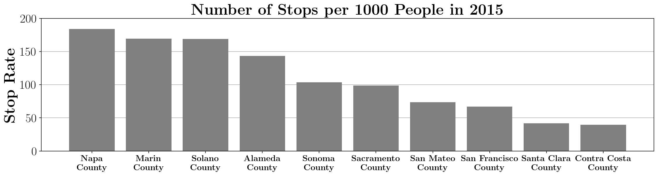 Figure 1: Stop rate in each Bay Area county
We can also examine the number of stops by race and violation, depicted in Figure 2. The majority of stops are of white drivers, followed by Hispanic drivers. At the same time, the majority of stops do not have a listed reason for the stop. Among listed reasons, “moving” violations a most common, while DUIs are only a small fraction of the stops.
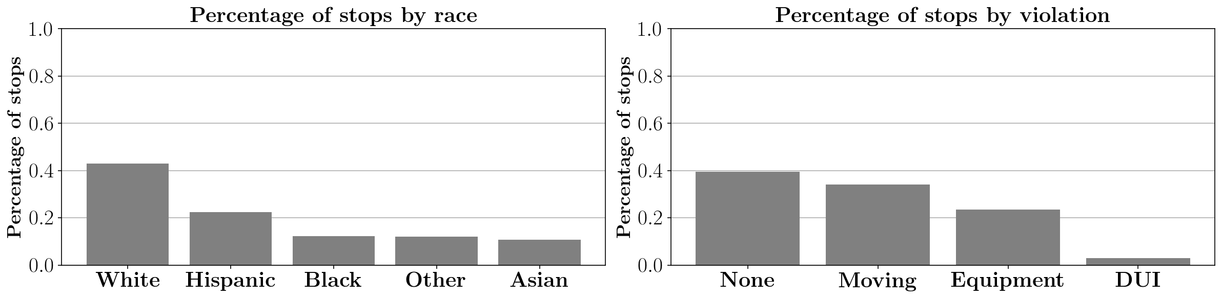 Figure 2: Fraction of stops by race (left) and violation (right).
Multilevel Model
I considered three separate models, each including more features than the previous model. For brevity, I’ll detail the complete model, and highlight which subset of variables was used for the prior models.
The complete model was a random intercepts logistic regression with interaction terms:
\begin{align}
&\text{logit}\{\text{Pr}(\texttt{search}_{ij}=1|\mathbf{x}_{ij}, \mathbf{z}_j)\} = (\beta_0 + \zeta_j) + \beta_1 \times \texttt{driver_male}_{ij} \\
&+\beta_2 \times \texttt{driver_black}_{ij} + \beta_3 \times \texttt{driver_hispanic}_{ij} \\
&+\beta_4 \times \texttt{driver_asian}_{ij} + \beta_5 \times \texttt{driver_other}_{ij} \\
&+\beta_6 \times \texttt{moving}_{ij} + \beta_7 \times \texttt{dui}_{ij} + \beta_8 \times \texttt{equipment}_{ij} \\
&+\beta_{9} \times \texttt{poverty_rate}_j + \beta_{10} \times \texttt{percent_nonwhite}_j \\
&+\beta_{11} \times \texttt{violent_crime}_j \\
&+\beta_{12} \times \texttt{driver_black}_{ij} \times \texttt{violent_crime}_j \\
&+\beta_{13}\times \texttt{driver_hispanic}_{ij} \times \texttt{violent_crime}_j
\end{align}
There’s a lot going on here, so let’s break it down. First, note that $i$ indexes the stop, while $j$ indexes the county.
Next, note the breakdown in variable terms:
- The first feature ($\beta_1$) controls for gender.
- The next four features ($\beta_2, \beta_3, \beta_4, \beta_5$) encode race. Hispanic refers to non-white hispanic.
- The next three features ($\beta_6, \beta_7, \beta_8$) encode the violation that led to the stop (e.g. moving violation, DUI, or equipment problem).
- The following four features are at the county-level ($\beta_9, \beta_{10}, \beta_{11}, \beta_{12}$) and respectively encode the population (in thousands), poverty rate (percentage of people below the poverty line), violent crime rate (number of violent crimes per 100,000 inhabitants), and property crime rate (number of property crimes per 100,000 inhabitants).
- The last two features encode interaction terms between race and crime rates.
Thus, the three models were as follows:
- Model 1: Baseline random intercept model.
- Model 2: Random intercept model with stop-level information (driver demographic information and violations).
- Model 3: Random intercept model with stop-level information and county-level features, including interaction terms.
Results
The three models detailed above were fit to the data using Stata. The resulting parameter estimates are depicted in Table 1. Note that all estimates are assumed to be significant at the $p=0.05$ level, except when denoted by a dagger.
$^{\dagger}$ denotes parameters that are not significant at the $p=0.05$ level.
| Model 1 | Model 2 | Model 3 | |
|---|---|---|---|
| Intercept | $-3.42 \ (0.06)$ | $-4.16 \ (0.06)$ | $-4.27 \ (0.20)$ |
| Male | $+0.39 \ (0.02)$ | $+0.38 \ (0.01)$ | |
| Black | $+0.73 \ (0.02)$ | $+0.35 \ (0.08)$ | |
| Hispanic | $+0.63 \ (0.02)$ | $+0.70 \ (0.05)$ | |
| Asian | $-0.24 \ (0.03)$ | $-0.24 \ (0.02)$ | |
| Other | $-0.35 \ (0.03)$ | $-0.34 \ (0.03)$ | |
| Moving | $+0.36 \ (0.02)$ | $+0.36 \ (0.02)$ | |
| DUI | $+1.83 \ (0.02)$ | $+1.83 \ (0.02)$ | |
| Equipment | $-0.05 \ (0.02)^{\dagger}$ | $-0.05 \ (0.02)$ | |
| Poverty Rate | $+0.04 \ (0.02)^{\dagger}$ | ||
| % Non-White | $-0.01\ (0.00)^{\dagger}$ | ||
| Violent Crime | $+0.02\ (0.03)^{\dagger}$ | ||
| Black x Crime | $+0.07\ (0.01)$ | ||
| Hispanic x Crime | $-0.01\ (0.01)^{\dagger}$ | ||
| Error Variance | $+0.18\ (0.04)$ | $+0.19\ (0.04)$ | $+0.13\ (0.03)$ |
The grand mean of the intercepts across the models were all large and negative, implying that searches do not occur often. In addition, the error variance for model 1 was $0.184$ with a residual intraclass correlation of $0.01$. This small ICC passes the likelihood ratio test at the $p = 0.001$ level, implying that a multi-level model is appropriate despite a small effect size.
In Model 2, we added individual level covariates including the driver’s violation and demographic information. The addition of these variables improved the likelihood while maintaining the small but significant residual ICC ($\hat{\rho}=0.01$). Importantly, the coefficients for black and Hispanic result in conditional odds ratios are $2.07$ and $1.88$, respectively. This implies that, given a county, they are more likely to be searched than a white driver (conversely, Asian and “Other” drivers are less likely to be searched than a white driver) given a stop. Thus, this provides evidence that there are racial disparities in search rates across the Bay Area but that they do not strongly vary across the Bay Area.
The complete model achieved the highest log-likelihood of the three models. In addition, it maintained the small but significant ICC ($\hat{\rho} = 0.005$). The inclusion of the interaction terms did not impact most of the individual level covariates except for whether the driver was black or Hispanic, as might be expected. The conditional odds ratios for black, hispanic, Asian, and other drivers are $1.42$, $2.01$, $0.79$, and $0.71$ compared to white drivers, respectively. Thus, the racial disparities among black and Hispanic drivers persist. Furthermore, it is worthwhile to note that the conditional odds ratio for male drivers $(1.47)$ implies that there may exist gender disparities, as the model implies that men are more likely to be searched than women. Among the violation variables, a DUI is the most significant with the highest effect size (conditional odds ratio of $6.25$), implying that drivers pulled over under the suspicion of DUI are much more likely to be searched.
In Model 3, all cluster-level covariates are not significant at the $p=0.05$ level. The Hispanic interaction term is also not significant, while the black interaction term is highly significant. Its conditional odds ratio is $1.074$, implying that among black drivers, each additional violent crime per 1,000 people results in a $7\%$ increase in the chance of a stop. This can result in a substantial increase in the likelihood that a black driver is pulled over depending on the county. Thus, violent crime rate among the Bay Area counties moderates the racial disparities of search rates among black drivers.
Context and Avenues for Future Work
Ideally, I would have operated at a finer spatial resolution (e.g. census tracts) as racial disparities are more likely to be moderated at this level (rather than the county level, which may blur the lines between segregated neighborhoods). Unfortunately, the dataset only provided stops at the county level. A study with data at the census tract level likely would have revealed correlations between socioeconomic factors at the cluster level and search rates, as past studies have shown. In contrast, our study did not observe strong variations among counties in the Bay Area, likely due to the small number of clusters and the large population in each county.
This analysis could have benefited from additional features, such as the driver’s age, ethnicity, the driver’s criminal history that was available to the officer, and for what reason the officer initiated a search. For example, past studies have examined such reasons in stop-and-frisk data and found that reasons such as “furtive movements” are often used but not predictive of a crime, thus providing a mechanism for which racial biases tie into frisk rates.
Furthermore, this analysis only assessed whether racial disparities existed in the decision to conduct a search given a stop, without regard for whether those decisions were correct (i.e. resulted in finding contraband). This is what is known as a benchmark test. Its main limitation is that it does not consider whether there are actual differences in the likelihood that members of different sub-groups will, for example, carry contraband. The recently proposed threshold test by Simoiu et al. [7] Simoiu, Corbett-Davies, Goel, The Annals of Applied Statistics, 2017. circumvents this issue by estimating the underlying distribution of likelihoods for different sub-groups using a latent Bayesian model.